



Many musical phenomena are periodic, including octave equivalence and rhythmic periodicity. Mathematics provides tools for modelling such structures: congruences. Take the melody below, for example: each note in this bar can be characterized by its position and pitch, represented by the horizontal and vertical axes respectively.
####
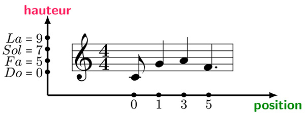
A first melody to be modelled.
A note’s position corresponds to the point at which it occurs in the bar—in other words, when it is played. The first note, C, occurs at time 0; time is then divided into suitably chosen units, and each subsequent note is assigned a number. This unit of time is usually based on the shortest note value—here, the eighth note—so that a quarter note counts for 2, a dotted quarter note for 3, etc. The bar therefore contains eight time units, meaning that we work "modulo 8."
Similarly, each note is assigned a pitch, corresponding in a sense to the "value" of the note being played in terms of frequency. In music analysis, pitches are often considered modulo a particular unit called the ambitus—the range of a melody, voice or instrument from its lowest to its highest note. Here, in particular, we focus on the number of octaves used to compose the melody: if all the notes lie within a single octave, comprising twelve notes, we work "modulo 12," with the convention that C has the value 0. Here we use enharmonic equivalence, meaning that C sharp is identified with D flat, D sharp with E flat, and so on.
Modelling musical events
---------------------------------
A melody is thus described by the positions of its notes within the bar and by their pitches, taken modulo the number of time units in a bar and the number of pitch classes in the octaves used. Mathematically, this information is modelled by treating the positions and pitches of the notes in a bar as subsets of a larger set: the set ℤ/nℤ of integers modulo n. In our example, we take n = 12 to indicate that we are working within a single octave, and n = 8 to indicate that the chosen time unit is an eighth note. This gives us two structures, P and H (positions and pitches), which can then be combined to give a periodic description (P, H) of the bar in terms of the notes’ positions and pitches.
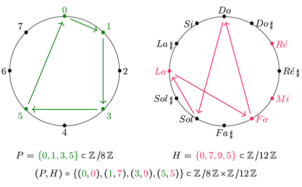
The preceding melody, represented by polygons and periodic structures.
Modelling the bars allows us to convert a piece into a point cloud: a set of points that can be compared using a distance measure. Consider a score from a piece of music. It is naturally divided into bars, each described in (ℤ/tℤ)×(ℤ/hℤ), where t is a unit of time and h is the pitch range we wish to use—that is, the number of octaves multiplied by 12. Each bar is therefore reduced to a single point (P, H) in the resulting point cloud. To compare them, we use the discrete Fourier transform. It was introduced by the composer and music theorist David Lewin (1933–2003) to characterize musical structures using, among other things, their periodicity, as measured by Fourier coefficients. We will use these same coefficients to calculate the distance between the bars of a piece of music.
If (P, H) represents a bar modulo t and h, and (x, y) is a note in that bar, where x is its position and y its pitch, then the associated Fourier coefficient is given by the following formula:
Each note yields one coefficient, while an entire bar yields a matrix—an array—of coefficients. Each score is thus divided into bars, which are assigned matrices of Fourier coefficients. The distance between the bars is then calculated from the distance between their associated matrices, naturally using a suitably chosen norm. This is how a score is turned into a point cloud.
Topology on musical scores
--------------------------------------
Using the model above, we can convert music into geometric—and more specifically topological—shapes: graph filtrations. A graph is an arrangement of vertices and edges, while a filtration is simply an increasing sequence of such objects. Given a score, each vertex represents one of its bars, and every pair of bars is assigned a distance via the Fourier transform. The distances are then ranked in increasing order, and the edges corresponding to each distance—and hence to each pair of bars—are added one by one. The filtration can also be made more complex by filling in certain triangles, tetrahedra and so forth according to a fixed rule, making it possible, for example, to add musical information. The resulting graphs are then called simplicial complexes. The point cloud constructed above forms the first stage of the filtration, which therefore has as many stages as there are distinct distances!

A graph filtration associated with a musical score.
The question now is: how can such objects be analysed? To do so, we use tools from topology. Topology is a branch of mathematics that studies everyday objects "up to deformation": imagine a cup made of modelling clay—it can be reshaped into a doughnut, whereas a basketball can never be transformed in this way and will always remain ball-shaped. An important task in topology, and particularly in algebraic topology, is to classify objects by assigning them topological invariants; homology provides one such invariant. It counts the "number of holes" or "loops" in every dimension of a given object: for example, an unfilled triangle has one hole in dimension 1, while a hollow sphere has one in dimension 2.
In our case, the aim is to measure this type of information in a graph filtration: in other words, we study how the loops formed during the filtration evolve. These features constitute the topological information we seek. The method is called persistent homology because we are interested in topological features that "persist" as the filtration progresses.
The evolution of homology in a filtration can easily be represented visually using diagrams called barcodes. If a loop appears at some stage t of the filtration—for example, when a triangle is formed—and disappears at time t + n—for example, when that triangle is filled in—we draw a bar of length n whose endpoints have x-coordinates t and t + n, respectively. In other words, each bar measures exactly how long a loop survives during the filtration, with the x-coordinates indicating when that loop appears and disappears. Put simply, these diagrams measure the topological information we wish to study in our filtration.
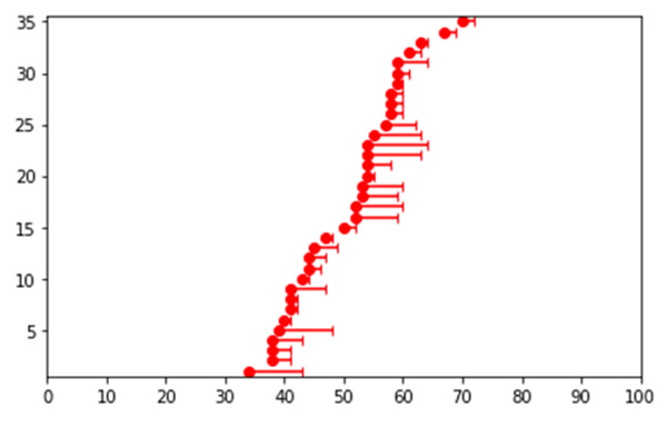
An example of a barcode.
Persistent homology and barcodes are powerful tools in topological data analysis, where several objects under study are characterized by topological signatures so that they can be analysed and compared. For example, persistent homology can be used in astronomy to classify constellations, or in medicine to compare arrangements of neurons.
Here, we propose using it in a slightly different setting: music analysis! How does this work in practice? The starting point of the thesis was to determine how a filtration of simplicial complexes could be associated with a musical score.
Once this process has been carried out, the next step is to study the associated barcodes. This allows scores to be analysed and, more specifically, compared.
By musical style
--------------------------------
A very common problem in the field of mathematics applied to music analysis is automatic style classification: creating an algorithm that takes a score as input, in the form of a MIDI file—short for musical instrument digital interface—and returns its musical genre—pop, rock, jazz and so on. Although the thesis has not yet produced systematic results, it offers promising avenues in this direction: by comparing the barcodes obtained for a selection of pieces, we were able to group artists and composers according to the style of the scores studied. The following figure illustrates the type of result obtained: it shows different clusters (groups) produced by comparing the composer Johann Sebastian Bach (1685–1750) with various groups and artists from the heavy metal, hard rock, pop and pop rock genres. For Bach, we studied a total of forty-five pieces, divided into three styles: fifteen preludes, fifteen fugues and fifteen chorales. For each artist, we selected fifteen pieces from their discography. In the charts, each colour represents an artist, and each point corresponds to a score from which a barcode was extracted. The legend shows statistics calculated directly from the barcodes to compare them: the mean bar length, standard deviation and entropy. This study is a first step towards the automatic classification of musical style!
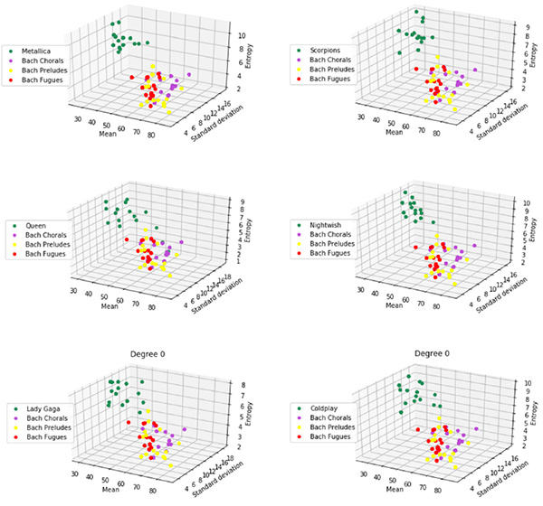
Classifying Johann Sebastian Bach alongside various groups and artists active
over the past fifty years.
Towards a large database
-----------------------------------
Many mathematical methods can help us understand music more fully, and the results presented here are only a very small illustration of their potential. In the field of classification, an enormous amount of work remains to be done, not least in extending this approach to a wider variety of musical styles, such as jazz and rap.
This requires more musical data to work with, and one part of the thesis involved starting to build a database of MIDI files, available at https://math-musique.pages.math.unistra.fr, which brings together the materials used and thus enables the community to work with them.
The thesis also examined other applications of topology to music, including Euler’s Tonnetz and the harmonization of pop songs. Mathematics still offers many musical applications waiting to be discovered and explored!