


Re-entry into the Martian atmosphere by the capsule carrying the Perseverance rover, weather forecasting, numerical simulation of a car crash, calculating an aircraft’s aerodynamic performance… Any numerical simulation begins with a modelling phase—physical, mechanical, biological or otherwise—which generally leads to complex mathematical equations. Except in textbook cases, these equations cannot be solved "by hand": numerical solution algorithms, themselves drawing on mathematics, are required. For example, simulating airflow around a car requires solving a system of millions of equations at every time step, taking hours even on a powerful computer.
High-performance computing
-----------------------------
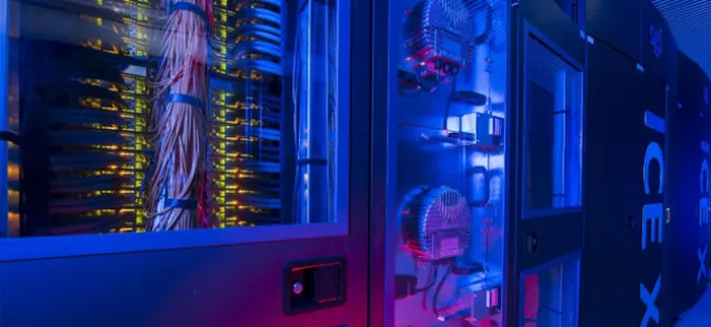
In the early 2000s, high-performance computing (HPC, short for high-performance computing), also known as supercomputing, was still limited to a handful of national research centers and large companies. A "supercomputer" was typically a cluster of hundreds of computers (known as compute nodes) connected by a very fast network. Such a system is obviously extremely costly, from its initial purchase through its cooling systems to its ongoing maintenance. Numerical simulations are distributed across the processors in the compute nodes. This is known as parallel computing.
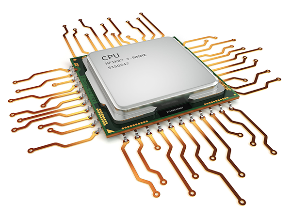
Over the past twenty years, both processor performance (CPUs, short for central processing units) and memory capacity have improved considerably, making even our personal computers far more powerful. Today, a CPU may itself contain several processing cores—typically four, eight, sixteen or even twenty—and each core can deliver 10 GFlops (ten billion floating-point operations per second). A twenty-core CPU can therefore reach an impressive theoretical peak performance of 200 GFlops, ignoring cache, latency and data-transfer effects and assuming that operations are perfectly balanced across the cores.