The ubiquitous normal distribution

In science, chance might be seen as an admission of weakness, a paradox, even a disreputable field! An admission of weakness because, since every effect has a cause, attributing an effect's occurrence to chance means failing to identify its cause correctly. A paradox because chance has laws of its own, the most famous being the normal distribution. And, finally, a disreputable field because it was scorned by pure mathematicians in the Bourbaki tradition. Yet the British physiologist Francis Galton (1822–1911) expressed his admiration for the order that arises from chance: "I know of scarcely anything so impressive as the wonderful form of cosmic order expressed by the Law of Frequency of Error… It reigns serenely and in complete self-effacement amidst the wildest confusion."

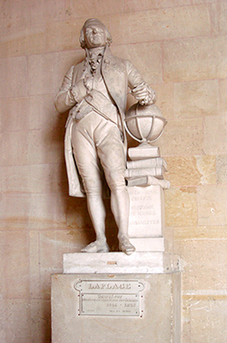
The "Law of Frequency of Error" is, of course, the normal distribution. Quantum physics has since introduced a form of chance that is necessary… and fundamental: God plays dice. For many years, the normal distribution was known as the Laplace distribution in France and the Gaussian distribution in English-speaking countries. Let us seek a consensus by calling it the Laplace–Gauss distribution, although the two mathematicians approached it differently…

Gauss: the astronomical route -------------------------------

Gauss devised the normal distribution to improve the astronomical observations made by his friend and colleague Heinrich Olbers. The German mathematician himself observed celestial objects only very occasionally, but he was interested in the positions of luminous objects, both to distinguish moving planets and asteroids from fixed stars (allowing for the Earth's rotation) and to calculate their trajectories. Gauss had therefore calculated the trajectory of Ceres, the first asteroid discovered (between Mars and Jupiter), from Olbers's observations. Olbers subsequently detected a moving object in the region where Gauss's calculations predicted Ceres would be. It was the asteroid Pallas, which happened to be passing close to Ceres. How can the position A of a celestial body best be determined from several measurements *A₁, A₂… A_n? The difference A_i – A between measurement number i and the true position is the error in the measured position of the celestial body. To calculate A, Gauss invented the celebrated method of least squares, which consists in calculating the value of A that minimizes the sum of the squares of the different values A_i – A. He showed that this value is the mean A_moy of the n observations A₁, A₂… A_n. Gauss also considered how the errors are distributed around the mean and proposed another method of calculation. Assuming that the errors are independent, he denoted by P(x_i) the probability of making the error x_i = A_i – A in the observation A_i. He then introduced the likelihood function V(A), equal to the product of the probabilities P(x_i), which is the probability that this series of errors occurred in the measurements. He made two assumptions: the function P is symmetric about the value A_mo*_y (the probability of measuring a particular value below A_moy equals the probability of measuring the corresponding value above it), and it decreases as the absolute value of the error *A_i – A_moy* increases. Gauss proved that the functions satisfying these two conditions are those of the form