


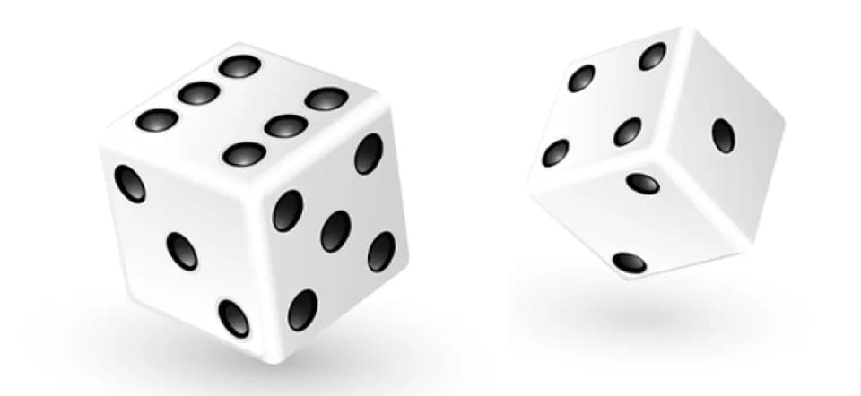
One of the best-known situations in probability theory is the roll of a fair die. We represent it by the set Ω = {1, 2, 3, 4, 5, 6} of possible outcomes of the experiment. To calculate the probability of rolling an even number, for example, we first determine how many elements of Ω are even (there are three), then divide this by the total number of elements in Ω (six in this case). The quotient 3/6, which simplifies to 1/2, is the probability we seek.
Early work in probability theory followed this purely counting-based approach, but it soon proved too restrictive. A die may, after all, be unbalanced (or loaded, as is sometimes assumed…), meaning that its center of mass does not coincide with the center of the cube, or that its faces are not quite identical. In that case, the elements of Ω do not all have the same chance of coming up. To cover this case, and more generally any situation in which the possible outcomes of a random experiment do not have the same chance of occurring, we need to go further.
One way to do this is to assign each element ω of Ω a value P(ω) corresponding to the probability that ω is the outcome of the roll. If, for example, the die lands on 6 twice as often as on any other face (which remain equally likely), then:
P(1) = P(2) = P(3) = P(4) = P(5) = 1/7 and P(6) = 2/7.
By assumption, the probabilities of rolling 1 through 5 are all equal to the same value p, while the probability of rolling 6 is 2p. We can then find p using one further assumption: probabilities add, just as in our first example the probability of the set {2, 4, 6} of even numbers was obtained by adding the probabilities of rolling 2, 4 and 6. Since the probability of the whole of Ω must equal 1 (that is, there is a 100% chance that the die will produce an outcome between 1 and 6), we have