



Integral calculus dates back to the ancient Greeks. In the 4th century BCE, Eudoxus of Cnidus was among the first to calculate areas by finding successively tighter bounds, using the method of exhaustion (see Le Calcul intégral, Bibliothèque Tangente 50, 2014). To bound the value of π, the Greeks—Archimedes foremost among them—inscribed a polygon of known area in a circle, then drew a second polygon outside the circle. Similarly, to calculate complex volumes such as that of a pyramid, they "cut them into thin slices." Differential calculus, by contrast, studies the rates at which quantities change. Although it is the inverse of integral calculus, it did not emerge until 2,000 years later.
The subtangent
----------------
Florimond de Beaune (1601–1652), a jurist and councillor at the Parlement de Blois (Loir-et-Cher), was one of the first commentators on Descartes's La Géométrie. At one point in his correspondence with René Descartes and Marin Mersenne, he proposed a problem: to determine a curve from a property of its tangent. This question was soon recast as that of finding a curve whose subtangent is constant at every point (the Florimond de Beaune problem). Descartes could find no general method; unable to give an algebraic expression for the curve, he proposed a mechanical construction. The "logarithmic curve" did not become known to mathematicians until around the end of the 17th century (see our feature "Les merveilles des logarithmes," Tangente 177, 2017), notably through the work of Christian Huygens, who named the curve, though he hesitated between "logarithmic curve" and "logistic curve."
Gottfried Wilhelm Leibniz (1646–1716) gives a solution to the problem in a paper published in 1684 that lays the foundations of differential calculus. In it, he demonstrates the power of this new tool, noting that his method applies to every curve, whether algebraic or transcendental. In particular, it makes it possible to solve what he identifies as "the inverse problem of tangents."
Drawing heavily on Pascal, Leibniz first defines the characteristic "triangle" (shown here in Guillaume de l'Hospital's somewhat more accessible presentation). M is a point on the curve. The line MT is tangent to the curve at M and meets the axis at T, while m is a point on the curve "infinitely close" to M. The segment Mm therefore "virtually coincides" with the short arc .