



Predicting changes in the size of an animal, plant or human population has enormous implications. Mathematics can help us model such situations. At first, sequences might seem appropriate, with each term *un representing, for example, the size of a population after n* years. This is true for some insects whose adults die in winter while their eggs wait for warmer days before hatching, or for certain plants whose seeds wait until spring to begin germinating. In these situations, the different generations are clearly distinct.
The situation becomes considerably more complicated when generations can overlap—that is, when adults of different ages can coexist. Add species such as humans, whose reproductive period follows no seasonal cycle, and sequences become unmanageable. Ideally, the situation should instead be modeled by a function N of time t. Observations of real-world situations suggest that the population growth rate, given by N’(t), also depends on the size of the population itself. In other words, N and N’ are related: this is where differential equations come in!
A simplistic model
-------------------
In 1798, Thomas Malthus, a pastor responsible for poor relief, published his Essai sur le principe de la population (An Essay on the Principle of Population). He suggested that the population growth rate depends on the birth rate b and death rate d, which he regarded as constants. The population therefore has an overall growth rate r = b – d, giving the relation N’ = rN. This is perhaps the simplest differential equation of all, and solving it explicitly gives N(t) = N0 exp(r t), where N0 is the initial population.
As intuition would suggest, if the birth rate exceeds the death rate, r is positive and the population grows. Conversely, if r < 0, the population decreases; if r = 0, births and deaths balance out and the population remains stable.