



Mathematical reasoning can sometimes offer solid reassurance, even in the most unexpected fields. Faced with the ravages of Covid-19 in these difficult and uncertain times, a rational picture based on realistic assumptions provides reasoned answers to some of the questions on everyone’s mind. Although no one can grasp all the social and economic consequences of the pandemic currently raging, modelling the phenomenon is immensely valuable in explaining or justifying certain measures, such as lockdown or quarantine. Admittedly, modelling necessarily involves some degree of simplification and therefore always relies on a series of simplifying assumptions whose validity cannot be taken for granted. This must be borne in mind both when drawing conclusions and when making decisions. It is even more important for an epidemiological phenomenon such as Covid-19, for which reliable or comprehensive data remain virtually unavailable.
The SIR model
-------------
Several epidemiological models have been developed to date. The simplest are compartmental models, which already shed particularly revealing light on certain aspects of the pandemic we are currently experiencing. The SIR model belongs to this category.
Let P be a population of n individuals, where n is large. We first assume that there is no initial immunity whatsoever in P. This was indeed the case with Covid-19: no vaccine was available when it emerged, and the immune systems of those affected had never encountered the new virus and had therefore not yet been able to respond. We also assume that all individuals are similar. This assumption is obviously not satisfied in practice, but since the reasoning concerns a large population, an analysis based on averages is still informative.
We divide the population into three groups: susceptible people, S (for “susceptible”); infected people, I (for “infectious”); and, finally, recovered people, R (for “recovered”). Together, these initials form the acronym SIR.
The compartments can of course be defined more finely. We can add a category for those who have died, D (for "dead"), and a group of infected people placed in quarantine, Q, who consequently no longer pose a risk to the susceptible population. For now, the main aim is to visualize how infections evolve when no measures are taken and the virus is allowed to spread freely.
SIR models may be discrete or continuous. In a discrete setting, we record the numbers in the various compartments at each time step (days or weeks). At time 0, the population distribution is assumed to be known: S has cardinality n − 1, I contains one individual, and R is empty. We then assume that during each time interval, every infected individual can infect any person in compartment S with some probability p. After each unit of time, an infected individual recovers (or dies) and therefore moves from I to R (or D). The model is thus stochastic and can potentially produce a great many different outcomes. To illustrate how the compartments evolve, the International Statistical Institute (ISI, an organization founded in 1885 and independent of any government) circulated among all its members an excellent presentation on the subject by Professor Tom Britton (Stockholm University), which is available online. This statistician devised a large-scale simulation study incorporating different values of the pair (n, p). One model parameter proves crucial to the conclusions: the basic reproduction number, namely the number of people in P whom each infected person can infect. Britton initially estimates this parameter using the approximate relation R 0 ≈ (n − 1) p ≈ np, using a large P and a small p.

The mathematician Tom Britton.
Two main cases arise. When R 0 is less than or equal to 1, no epidemic breaks out. The proportion of people infected never exceeds 10%. But as soon as the basic reproduction number R 0 exceeds 1, two scenarios emerge. Either the virus quickly dies out after infecting only a small number of people (less than 10%), or a critical percentage of the population becomes infected. Thus, for R 0 = 1.5, a large number of simulations yield an infection rate of around 60%. By contrast, intermediate rates of between 10% and 50% are never observed. This phenomenon can be explained. Let τ denote the final proportion of the population infected over the course of the pandemic. The total number of individuals who have passed through category I is therefore nτ. The proportion of the population not infected by the virus is clearly 1 − τ. Within the model, this quantity can be viewed as a probability: specifically, the probability of not having been infected by any of the nτ individuals who carried the virus during the epidemic. If infections are independent events, we can write 1 − τ = (1 − p) *n*τ.
It remains to replace p with the value derived from the estimated basic reproduction number, namely p = R 0 / n. This gives the expression whose well-known limit as n tends to infinity is exp(− R 0τ).
Estimating R0
-----------------------------
The equation to be solved is therefore 1 − τ − exp(−R 0τ) = 0. Let f (τ) denote its left-hand side. The equation always has the trivial solution τ = 0. Indeed, this is its only solution for every value of R 0 less than or equal to 1. For values of R 0 strictly greater than 1, however, a second, positive solution appears, as shown in the following graph of the function f (τ) for R 0 = 1.5.
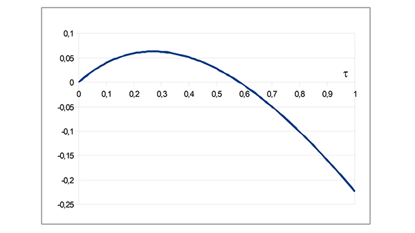
Graph of the function f for R0= 1.5.
The second solution (τ ≈ 58%) agrees perfectly with the simulation results. There is no explicit expression for the general solution, but the numerical calculations are straightforward and produce the following graph, which estimates the population’s infection rate τ as a function of the basic reproduction number R 0. The increase is rapid once R 0 moves away from the threshold value 1. For Covid-19, various sources estimate R 0 to be between 2 and 2.5, suggesting that without public action or preventive measures, the infection rate would be around 80%.
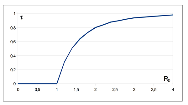
Estimated value of τ as a function of R0.
The effect of the measures
-------------------
The situation is of course entirely different when part of the population is immune or vaccinated. Suppose that a proportion q of the population is immune or vaccinated. Only the remaining proportion 1 − q can become infected. Our equation now becomes 1 − τ = q + (1 − q) exp(− R 0τ).
Now imagine that half the population is vaccinated (q = 1/2). For values of R 0 less than or equal to 2, the new equation then has only the solution τ = 0. The model thus confirms quantitatively that mass vaccination is the way to prevent the virus from returning and causing a second pandemic. The following graph compares the situations without vaccination (in blue) and with vaccination (in red) for q = 0.5.
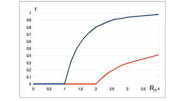
τ as a function of R0, with (in red) and without (in blue)
mass vaccination of the population.
We are not there yet. So what can we do to combat what at first seems inevitable? It seems reasonable to assume that the basic reproduction number must be proportional to the probability of transmission through contact. This is the case in the SIR model above: R 0 = np. We can reduce this probability by wearing masks and washing our hands; both measures affect p.
But the reproduction number just as clearly depends on how many contacts each person makes. We can therefore reduce R0 in a second way: by keeping a large proportion of the population at home and banning meetings and public gatherings.
Other factors also come into play, such as the population’s testing rate. In the case of Covid-19, some countries, including Germany, conduct mass testing. Others, such as Belgium, tested only patients in a worrying condition who displayed symptoms of the disease during the first few weeks, along with healthcare workers… provided they had a fever! The sizes of populations S and I are therefore unknown, making it impossible to determine a credible death rate. Compartment R consequently includes both those who have recovered and those who have died. Subsequent statistics will probably allow the death rate to be quantified accurately. This illustrates the value of initiatives such as the Polymath project.
What should we take away from all this? First, that appropriate measures can be adopted and must reduce the basic reproduction number. This is where mathematical models prove their worth: they quantify the consequences of our actions. As decision-making tools, they justify certain difficult measures. Finally, they offer reassurance about the future. What more could we ask?