



These are parametric curves of the form x = f (t ), y = g (t ), where f and g are piecewise cubic polynomials. Any curve can be approximated by Bézier curves so closely that the difference from the ideal curve is invisible to the naked eye.
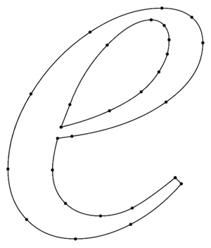
An italic "e" typeset using twenty-eight Bézier curves.
One problem is how to draw a curve of constant width 2r. The geometric solution is simple: take a curve L, then have the center of a circle of radius 2r trace that curve. The region swept out by the circle is the desired constant-width line.
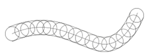
Analytically, it is another matter altogether. If the centerline L of the thick line is defined by the parametric equations x = f (t ) and y = g (t ), the boundary of the line of thickness 2r is the envelope of the circles of radius r centered on the centerline.
It is given by an expression of the form:
With the square root of a polynomial of degree 4 in the denominator, this is a far cry from Bézier curves. To "fit the envelopes into the system," another approximation is needed. Knuth's idea is to replace the circle with a regular octagon.
The visual difference is minimal. The main advantage is that the point that traces out the envelope (as the center of the octagon traces L) stays at one vertex of the octagon before shifting to another. While the tracing point stays at a given vertex, the envelope is very easy to calculate: it is a translate of the centerline L. Like L, the envelope is therefore a piecewise cubic curve.