



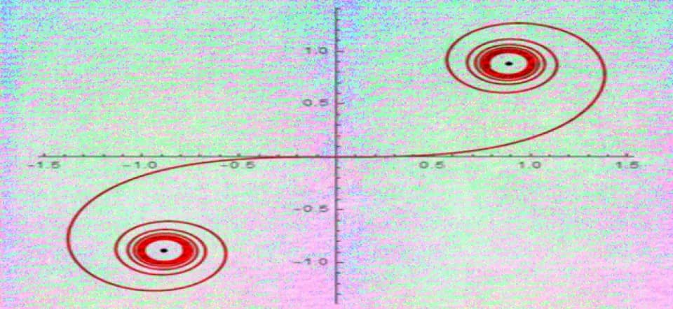
A parametrized curve is defined by the position of a point M(t) on the curve as a function of a parameter, often denoted by t because historically it represented time. The coordinates (x,y) of M are therefore functions of t: we can write x = f (t) and y = g (t), where f and g are real-valued functions. Depending on the case, they may be continuous, of class C1 (their derivatives exist and are continuous), of class C *n (their derivatives up to order n* exist and are continuous), of class C∞ (derivatives of every order exist and are therefore continuous) …
To avoid overly "pathological" curves such as those of Peano and Lebesgue (see the article "A precise definition? Not so simple!"), we shall consider only cases in which f and g are at least of class C1 on their domains. In practice, class C2 is generally enough to study a curve satisfactorily, whether its local behavior (tangent, center and radius of curvature, inflection point, etc.) or its overall shape (variation, infinite branches, convexity, etc.). Let us look at an important special case. Given a real-valued function f of a real variable, we often want its graph—that is, the curve with equation y = f (x). This is a special case of a parametrized curve: such a curve can be defined by x (t) = t and y (t) = f (t), where t is the parameter. Studying a parametrized curve is relatively straightforward, as is drawing it once the analysis is complete. Moreover, since the advent of digital tools (computers, graphing calculators, etc.), it can be plotted point by point without any prior analysis. We must therefore take care not to confuse the notion of a parametrized curve with its graph!
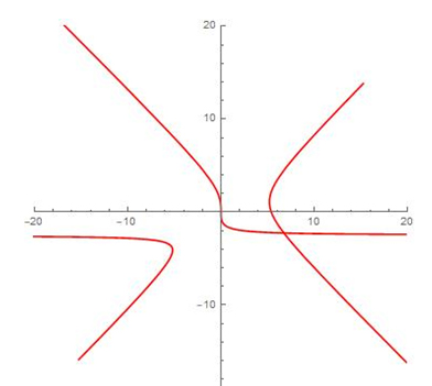
Graph of the curve defined by
and