



The trapezoidal rule
-----------------------

Let f be a positive continuous function defined on an interval \[a, b\]. The integral can be interpreted as the area between the graph of f and the x-axis (between a and b). Now draw the trapezoid bounded by the curve, the x-axis and the line segment \[AB\].
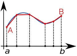
If the function f is reasonably smooth—that is, if its second derivative does not vary too much—the area of the trapezoid is close to the integral in question. We can approximate the integral by this area, namely (b – a)(f(a) + f (b)) / 2. Thus, if a = 1, b = 2 and f (x) = 1 / x, we obtain
which we approximate by (1 + 1 / 2) / 2 = 0.75.
The larger the interval and the greater the variation of the function over it, the larger the error. This suggests dividing the original interval into n equal parts, applying the method above to each of these n intervals, and adding the results. We thus obtain an approximation of
by setting h = (b – a) / n, as follows:
Returning to our example with n = 4, we obtain I4 = 0.6845, giving an error of less than one hundredth!
Rigour, of course, requires a theoretical upper bound on the error. If the function f is twice differentiable and its second derivative is bounded in absolute value by a number M, then the error itself is bounded above by M (b – a)3 / 8n2. In particular, if n tends to infinity, the error tends to 0, making it possible to obtain the result with an arbitrarily small error.
-
The double integral
------------------
If g is a real-valued function defined on a subset D of the plane, we can visualize it as the surface consisting of the points with coordinates (x, y, z) such that z = g (x, y) and (x, y) belongs to the domain D. By analogy with the integral over a line segment, if the function is positive, we want the integral over D to correspond to the volume between the plane {z = 0} and the surface above D. Such an integral can be constructed rigorously, subject to a few restrictions, but the process is… long and delicate (see le Calcul intégral, Bibliothèque Tangente 50, 2014).
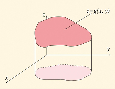
First consider the case where g is continuous and D = \[a, b\] × \[c, d\] is a rectangle. Since the function has two variables (x and y), we can first integrate with respect to x from a to b, then with respect to y from c to d, or the other way round. Miraculously, Fubini's theorem assures us that the two results agree and that the order of integration can indeed be reversed!