The circles of Apollonius of Perga: harmonic ratios

Harmonic ratios --------------------

It was during the baby-boom years. The bugbear of geometry in the second year of secondary school was to determine the locus of points M in the plane such that, for two given fixed points A and B, the ratio MA / MB is constant, equal to k. In those distant days, sadistic examiners asked this question in the oral examination for the first baccalaureate, guaranteeing an inevitable catastrophe. Of course, the equation of the locus is found analytically: MA² = k ²MB². For the points A($-a-a$, 0) and B($aa$, 0), after expansion, one obtains a circle centred on the line (AB) at

and with radius

$\text{R}={\displaystyle \frac{2ak}{\mathrm{\mid }{k}^2-1\mathrm{\mid }}}\backslash text\{R\}=\backslash dfrac\{2ak\}\{|k^2-1|\}$.

Descartes would certainly have been satisfied, but not the proponents of synthetic geometry.

At that time, when geometry reigned supreme, it was first shown that the angle bisectors of triangle MAB at M met the opposite side at points I and J such that IA / IB = JA / JB = k. Drawing through B the line parallel to side [AM], one then only has to apply Thales' theorem to triangles AIM and BII' and to triangles AJM and BJJ'.

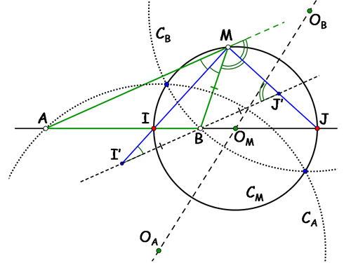
Since the angle bisectors are perpendicular, the sought locus is therefore the circle C_M with diameter [IJ]. The harmonic division [A, B, I, J] makes the pencil of lines (MA), (MI), (MB), (MJ) harmonic, but this was not taken into account in that proof.

The circle C_M, the locus of point M for fixed k, is called an Apollonius circle. The circles C_A and C_B are constructed in the same way using the angle bisectors at vertices A and B. These three circles have a common chord, and their centres are aligned on the Lemoine line. Numerous properties thus illustrate the geometric spirit of mathematicians of the late 19^th century, such as Henri Brocard, Émile Lemoine and Joseph Neuberg, among others.

-

Flux from the terminals ------------------

The electric field created by an infinite straight wire with linear charge density λ is radial, for reasons of symmetry, and has magnitude

for a point located at distance r from the wire. The associated potential V is given by

since the electric field is derived from its potential. If point M moves along an equipotential, we have

$d\text{V}=-\overrightarrow{E}\mathrm{.}\overrightarrow{d\text{M}}=0d\; \backslash text\{V\}=-\{\backslash overrightarrow\{E\}\}.\{\backslash overrightarrow\{d\backslash text\{M\}\}\}=0$.

The field line associated with the field $\overrightarrow{E}\{\backslash overrightarrow\{E\}\}$ is therefore orthogonal to the equipotential line.

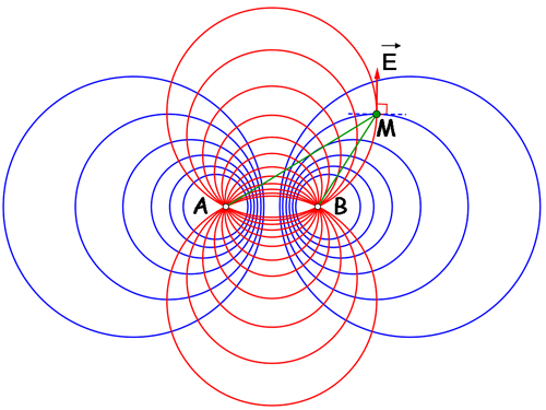
If we consider two wires perpendicular to the same plane, at A and B, with opposite linear charge densities, the potential is proportional to ln(r₂ / r₁ ) at a point M in the plane located respectively at distances r₂ and r₁ from the wires.

The equipotentials are therefore the curves for which r₂ / r₁ is constant. This is the bipolar definition of Apollonius circles, which form a pencil whose radical axis is the perpendicular bisector of [AB] (blue curves). The field lines are the orthogonal trajectories (red curves) of this pencil: they are circles passing through A and B whose centres lie on the perpendicular bisector of [AB].

Together, these curves form an orthogonal coordinate system parametrized by α and β: in a coordinate system with line (AB) as the x-axis and its perpendicular bisector as the y-axis,

and

where $aa$ is half the distance from A to B.

For fixed $\alpha \backslash alpha$, the blue circles have centre ($aa$ cot($\alpha \backslash alpha$), 0) and radius

and for constant β, the conjugate pencil of red circles, whose radical axis is the y-axis, has centre (0, $aa$ coth($\alpha \backslash alpha$)) and radius

${\displaystyle \frac{\alpha }{\sinh (\beta )}}\backslash dfrac\{\backslash alpha\}\{\backslash sinh(\backslash beta)\}$.

If the linear charge densities have the same sign, the equipotential lines are such that the product r₁r₂ is constant.

These are Cassini ovals, whose orthogonal curves are rectangular hyperbolas.

*

*